Time Series Method

Convert plotTS() Function to Use netCDF4 Parameters

import sys
!{sys.executable} -m pip install netCDF4
!{sys.executable} -m pip install xarray
import opedia
import netCDF4
import os
import json
import xarray as xr
from datetime import datetime
from netCDF4 import num2date, date2num
import numpy as np
import pandas as pd
import db
import common as com
import timeSeries as TS
from datetime import datetime, timedelta
import time
from math import pi
from bokeh.io import output_notebook
from bokeh.plotting import figure, show
from bokeh.layouts import column
from bokeh.models import DatetimeTickFormatter
from bokeh.palettes import all_palettes
from bokeh.models import HoverTool
from bokeh.embed import components
import jupyterInline as jup
if jup.jupytered():
    from tqdm import tqdm_notebook as tqdm
else:
    from tqdm import tqdm

Xarray Implementation

def plotTSX(tables, variables, startDate, endDate, lat1, lat2, lon1, lon2, depth1, depth2, fname, exportDataFlag, marker='-', msize=20, clr='purple'):
    p = []
    lw = 2
    w = 800
    h = 400
    TOOLS = 'pan,wheel_zoom,zoom_in,zoom_out,box_zoom, undo,redo,reset,tap,save,box_select,poly_select,lasso_select'
    for i in tqdm(range(len(tables)), desc='overall'):
        dt = 1     
        unit = tables[i].variables[variables[i]].attrs['units']
        
        toDateTime = tables[i].indexes['TIME'].to_datetimeindex()
        tables[i]['TIME'] = toDateTime
        y = tables[i].sel(TIME = slice(startDate, endDate), LAT_C = slice(lat1, lat2), LON_C = slice(lon1, lon2), DEP_C = slice(depth1, depth2))
        t = y.variables['TIME'].values
        y = y.variables[variables[i]][:,0,0,0].values.tolist()
        
        if exportDataFlag:
            exportData(t, y, yErr, tables[i], variables[i], lat1, lat2, lon1, lon2, depth1, depth2)
        
        output_notebook()
        p1 = figure(tools=TOOLS, toolbar_location="above", plot_width=w, plot_height=h)
        p1.xaxis.axis_label = 'Time'        
        p1.yaxis.axis_label = variables[i] + str(unit)
        leg = variables[i]
        fill_alpha = 0.3        
        cr = p1.circle(t, y, fill_color="grey", hover_fill_color="firebrick", fill_alpha=fill_alpha, hover_alpha=0.3, line_color=None, hover_line_color="white", legend=leg, size=msize)
        p1.line(t, y, line_color=clr, line_width=lw, legend=leg)
        p1.add_tools(HoverTool(tooltips=None, renderers=[cr], mode='hline'))
        
        
        p1.xaxis.formatter=DatetimeTickFormatter(
                hours=["%d %B %Y"],
                days=["%d %B %Y"],
                months=["%d %B %Y"],
                years=["%d %B %Y"],
            )
        p1.xaxis.major_label_orientation = pi/4

        p.append(p1)
    dirPath = 'embed/'
    if not os.path.exists(dirPath):
        os.makedirs(dirPath)        
    #if not inline:      ## if jupyter is not the caller
    #   output_file(dirPath + fname + ".html", title="TimeSeries")
    show(column(p))
    return

Testing Space

#TESTS XARRAY IMPLEMENTATION

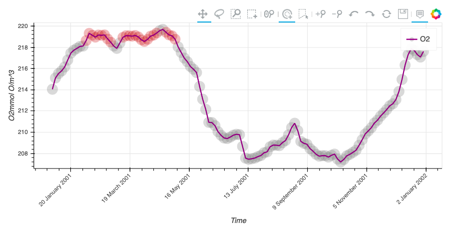
xFile = xr.open_dataset('http://3.88.71.225:80/thredds/dodsC/las/id-a1d60eba44/data_usr_local_tomcat_content_cbiomes_20190510_20_darwin_v0.2_cs510_darwin_v0.2_cs510_nutrients.nc.jnl')

tables = [xFile]    # see catalog.csv  for the complete list of tables and variable names
variables = ['O2']                                        # see catalog.csv  for the complete list of tables and variable names
startDate = '2000-12-31'
endDate = '2001-12-31'
lat1, lat2 = 25, 30
lon1, lon2 = -160, -155
depth1, depth2 = 0, 10
fname = 'TS'
exportDataFlag = False      # True if you you want to download data

plotTSX(tables, variables, startDate, endDate, lat1, lat2, lon1, lon2, depth1, depth2, fname, exportDataFlag)